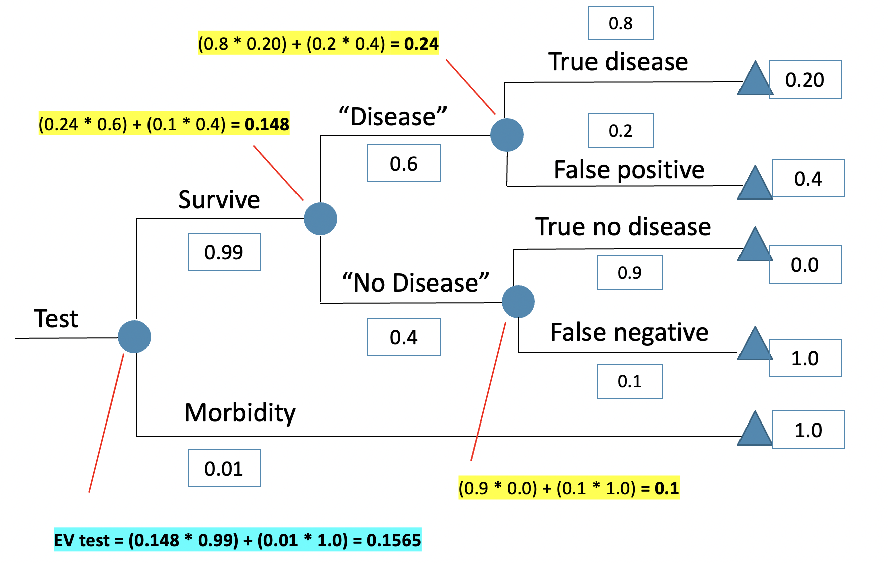
Structure of a Decision Analysis
Decision Trees & Probabilities
Should I go to the beach or stay home?
Possible States of the World:

At the beach with no rain.

At the beach with rain.

At home with no rain.

At home with rain.
Should I go to the beach or stay home?
Considerations:
Probabilities

Likelihood of Rain
Payoff

My overall well being in each state.
Should I go to the beach or stay home?
Considerations:
Probabilities
Likelihood of Rain
Payoff
Mood when it is sunny at the beach
Payoff
Mood when it is raining at the beach
Payoff
Mood when it is sunny at home
Payoff
Mood when it is raining at home
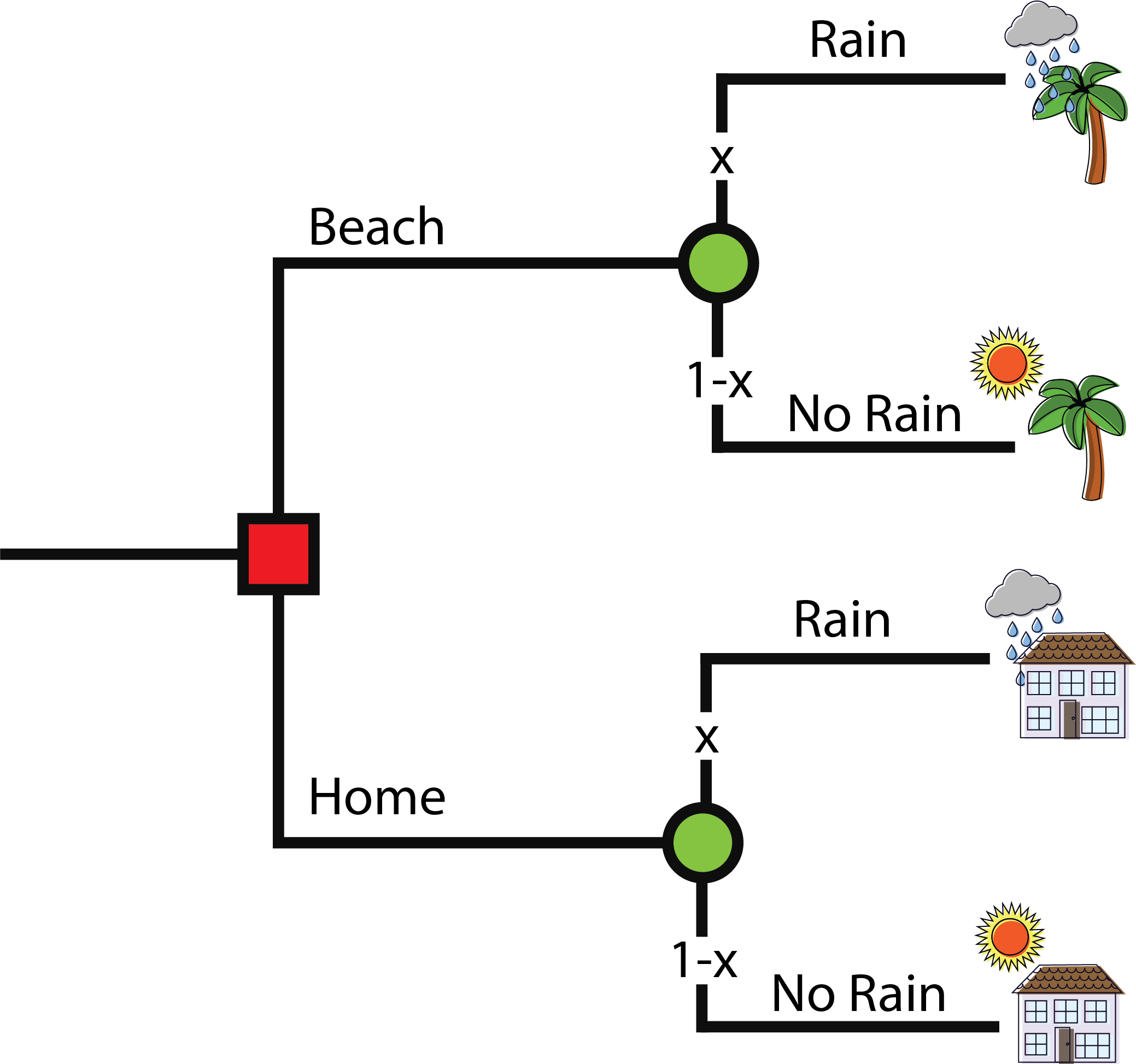
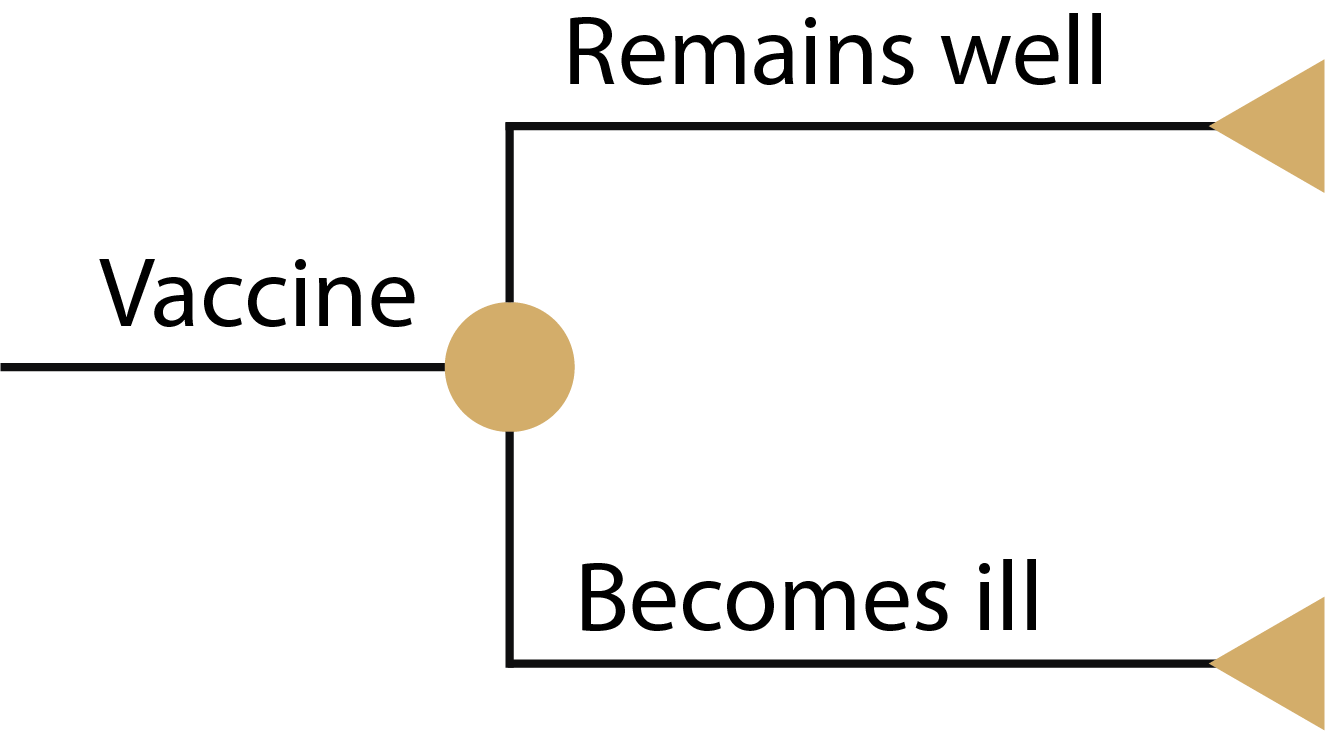
Decision Trees
Square decision node
- Indicates a decision point between alternative options

Circular Chance Node
- Shows a point where two or more alternative events for a patient are possible

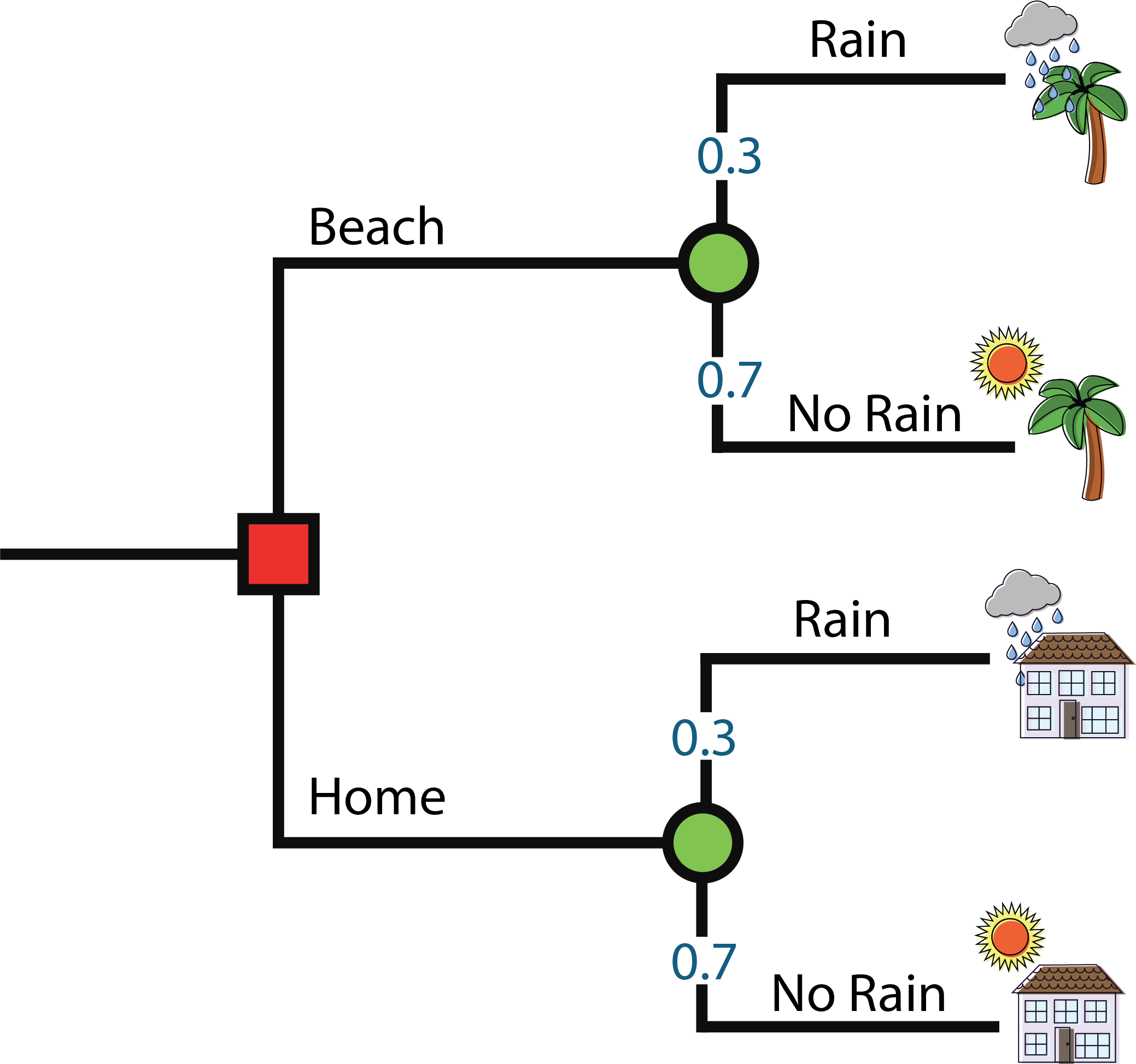
Should I go to the beach or stay home?
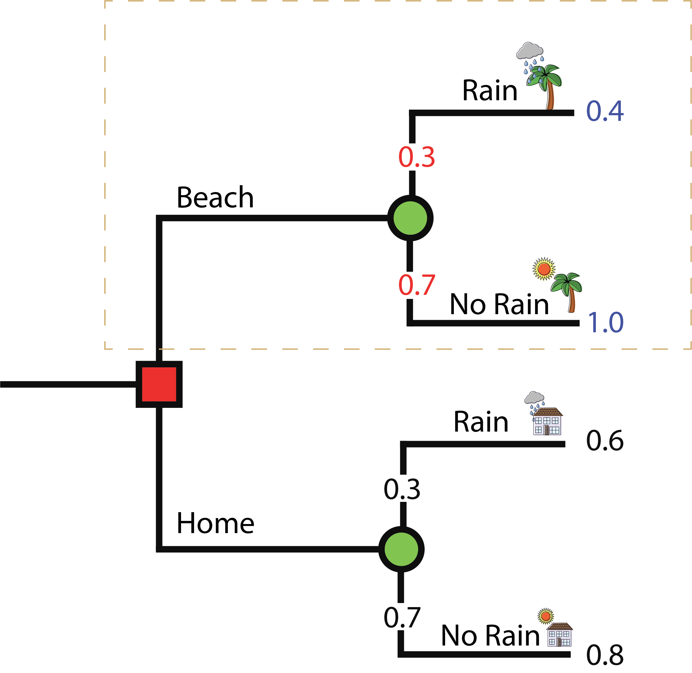
Decision Tree:
Probability of rain = 30%
Should I go to the beach or stay home?
Decision Tree:
Should I go to the beach or stay home?
Payoffs
| Scenario | Payoff |
|---|---|
| At beach, no rain |
1.0 |
| At beach, rain ↓ |
0.4 |
| At home, no rain ↑ |
0.8 |
| At home, rain ↑ |
0.6 |
| Scenario | Payoff |
|---|---|
| At beach, no rain BEST |
1.0 |
| At home, no rain |
0.8 |
| At home, rain |
0.6 |
| At beach, rain WORST |
0.4 |
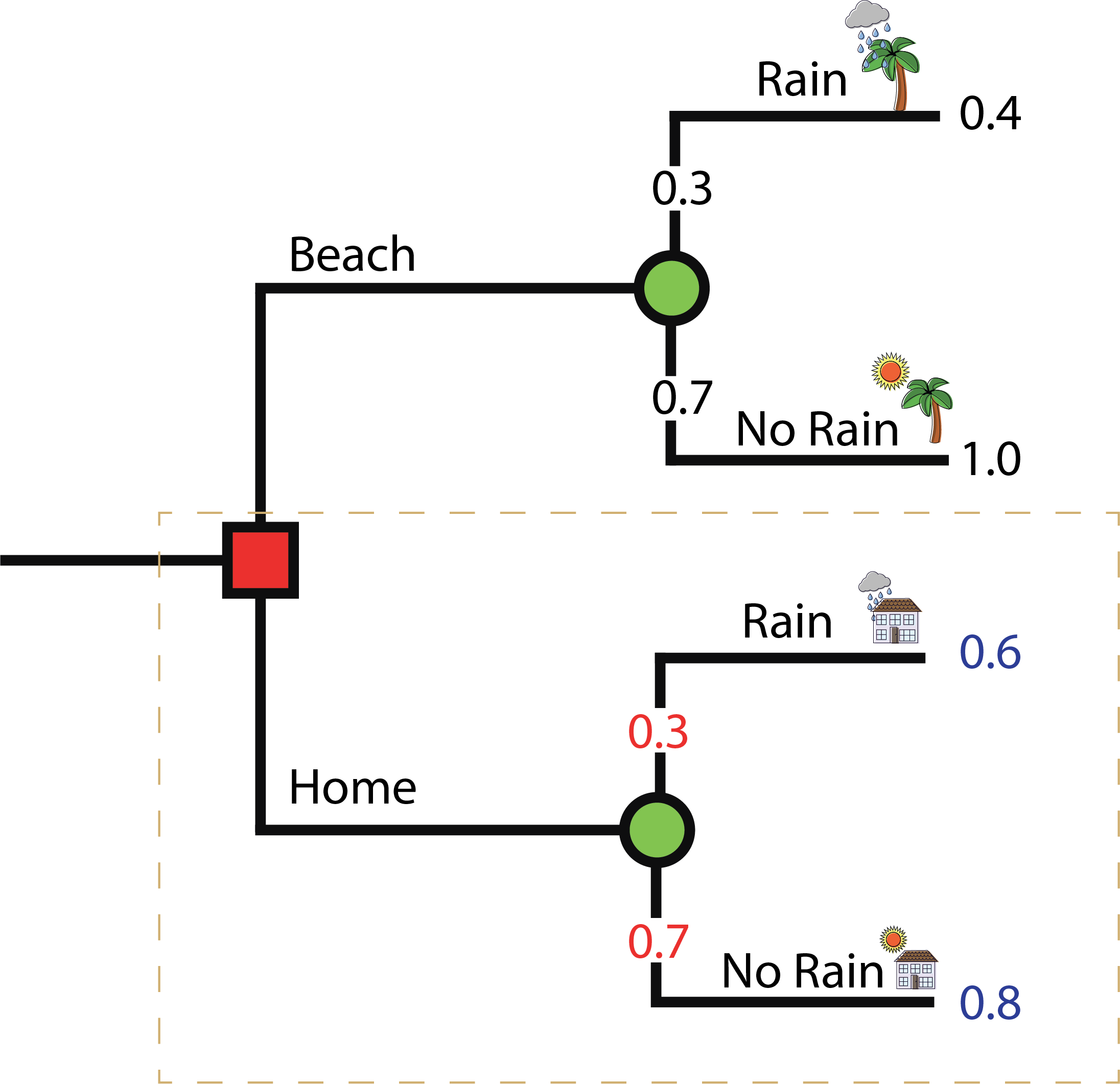
Should I go to the beach or stay home?
Decision Tree:
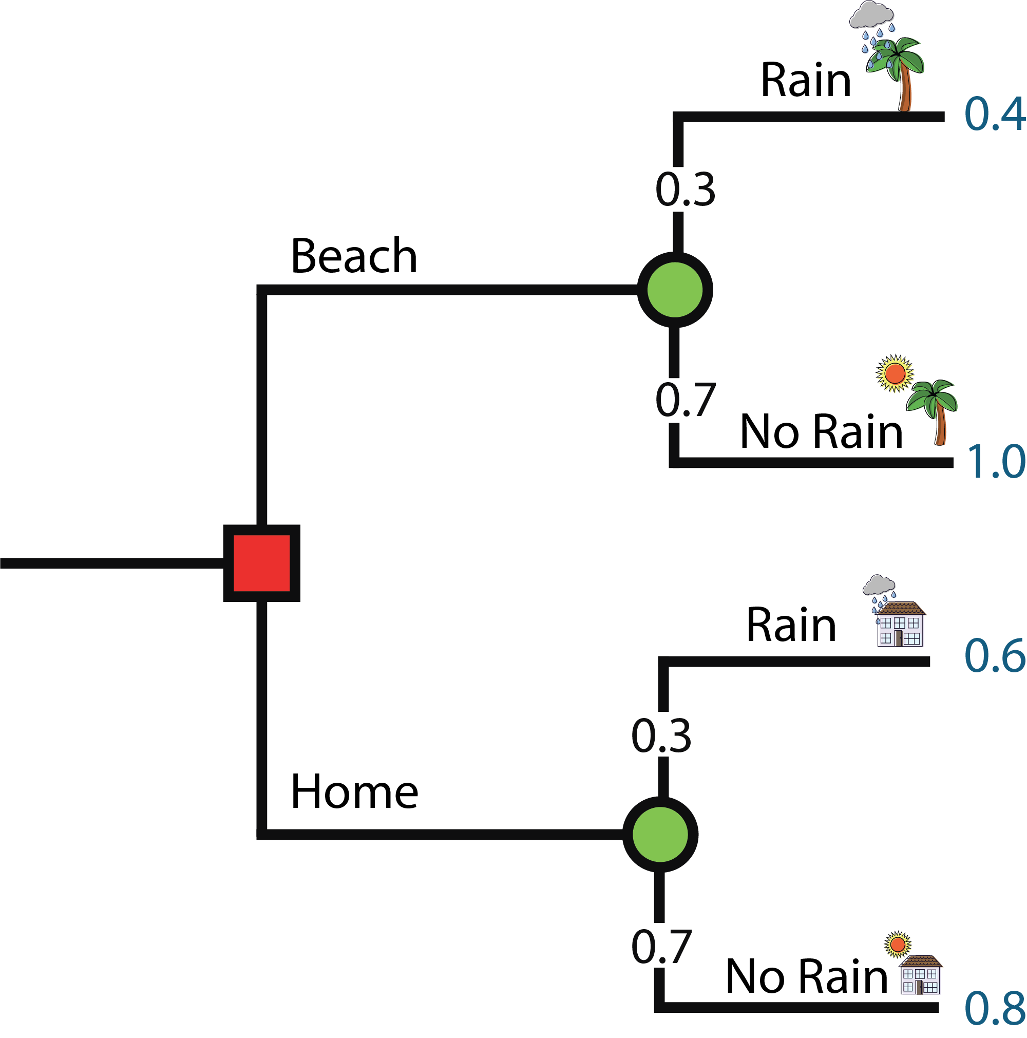
What is the expected value of going to the beach?
\color{green}{0.82} = \underbrace{\color{red}{0.3} * \color{blue}{0.4}}_{\text{Rain}} + \underbrace{\color{red}{0.7} * \color{blue}{1.0}}_{\text{No Rain}}
- Probabilities in red.
- Payoffs in blue.
- Expected value in green.
What is the expected value of staying home?
\color{green}{0.74} = \underbrace{\color{red}{0.3} \cdot \color{blue}{0.6}}_{\text{Rain}} + \underbrace{\color{red}{0.7} \cdot \color{blue}{0.8}}_{\text{No Rain}}
- Probabilities in red.
- Payoffs in blue.
- Expected value in green.
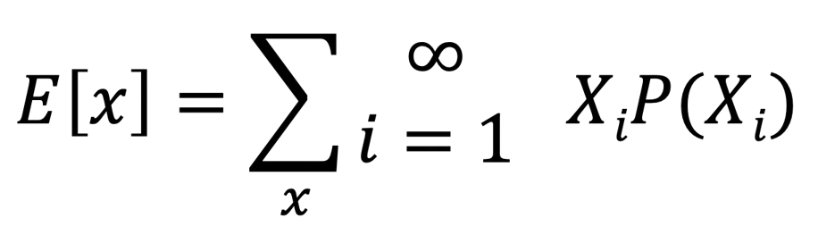
Expected Values
- Expected value = The sum of the multiplied probabilities for each chance option or intervention
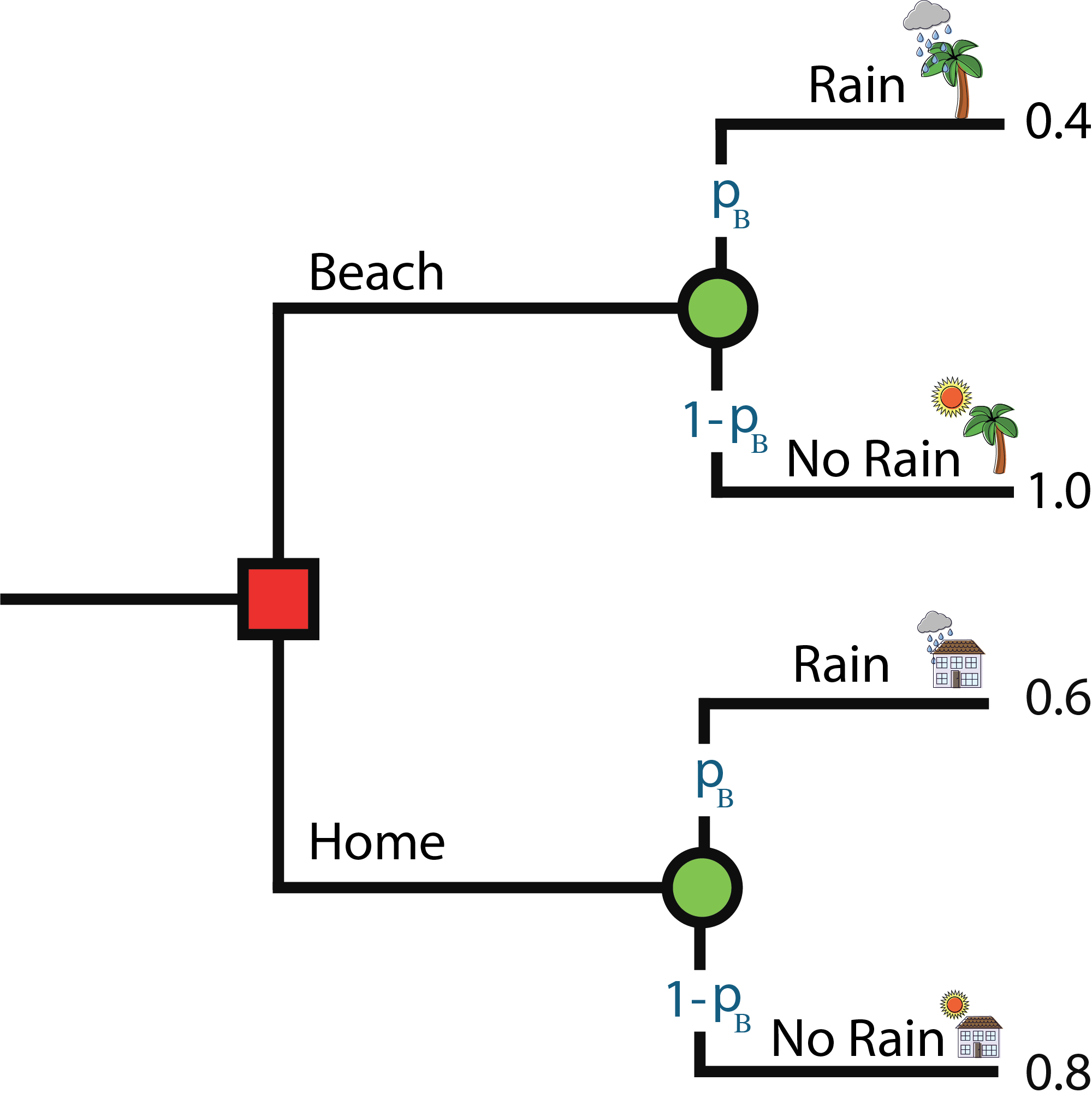
At what probability (p_B) of rain for the beach are you indifferent between the two options?
Mutually exclusive events in Decision Trees
Probabilities
- Moving from left to right, the first probabilities in the tree show the probability of an event.
- Subsequent probabilities are conditional. The probability of an event given that an earlier event did or did not occur.
- Multiplying probabilities along pathways estimates the pathway probability, which is a joint probability.
Decision Tree
Pathways
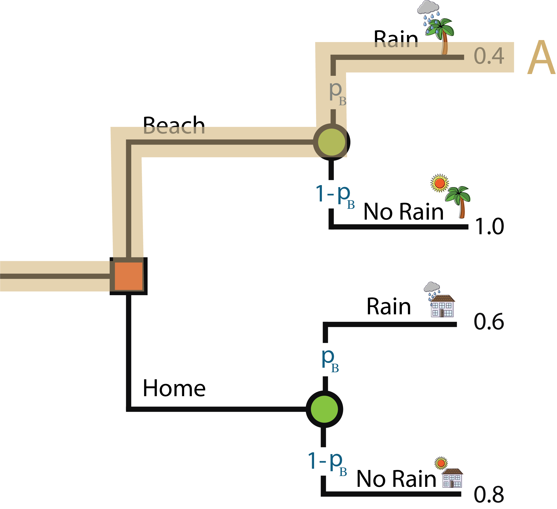
Pathway A: This person goes to the beach but it rains
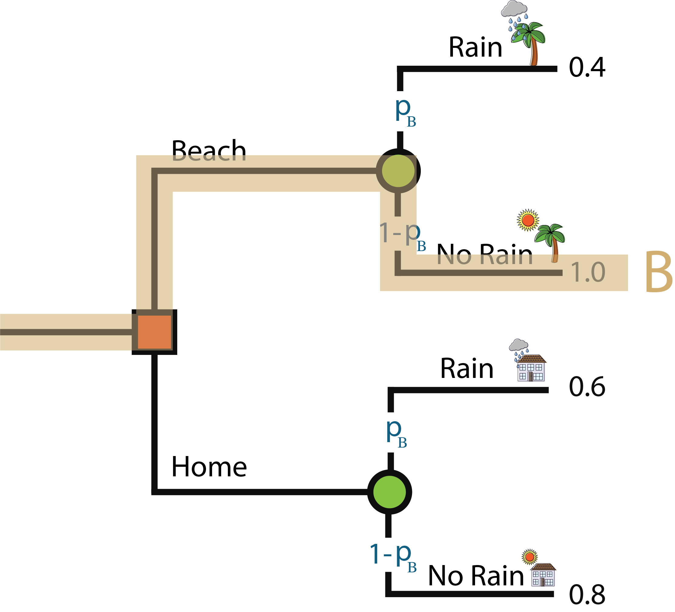
Pathway B: This person goes to the beach but there is no rain
Conditional probability, 2x2 review
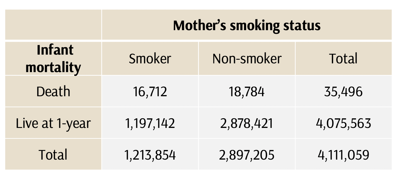
What is the conditional probability of death within a year of birth, given the infant has a mother who smokes?
P(A|B)
= P(death in first year | mother who smokes)
= 16,712 / (1,197,142 + 16,712)
= 14 per 1,000 births
Conditional probability, 2x2 review
Or, if we wanted to use the conditional probability equation
P(A|B) = P(A and B)/P(B)
*A= death in first year; B=mother who smokes
P(A and B) = 16,712 / 4,111,059 = 0.0041
P(B) = 1,213,854/4,111,059 = 0.295
P(A|B) = 0.0041/0.295 = 0.014
Conditional probability, A|B vs B|A
Probability of A|B is different from that of B|A
If A = death in first year; B=normal birth weight infant,
THEN, the conditional probability of P(A|B) = the probability of an infant death, given that the child has a normal birth weight
Conditional probability, A|B vs B|A
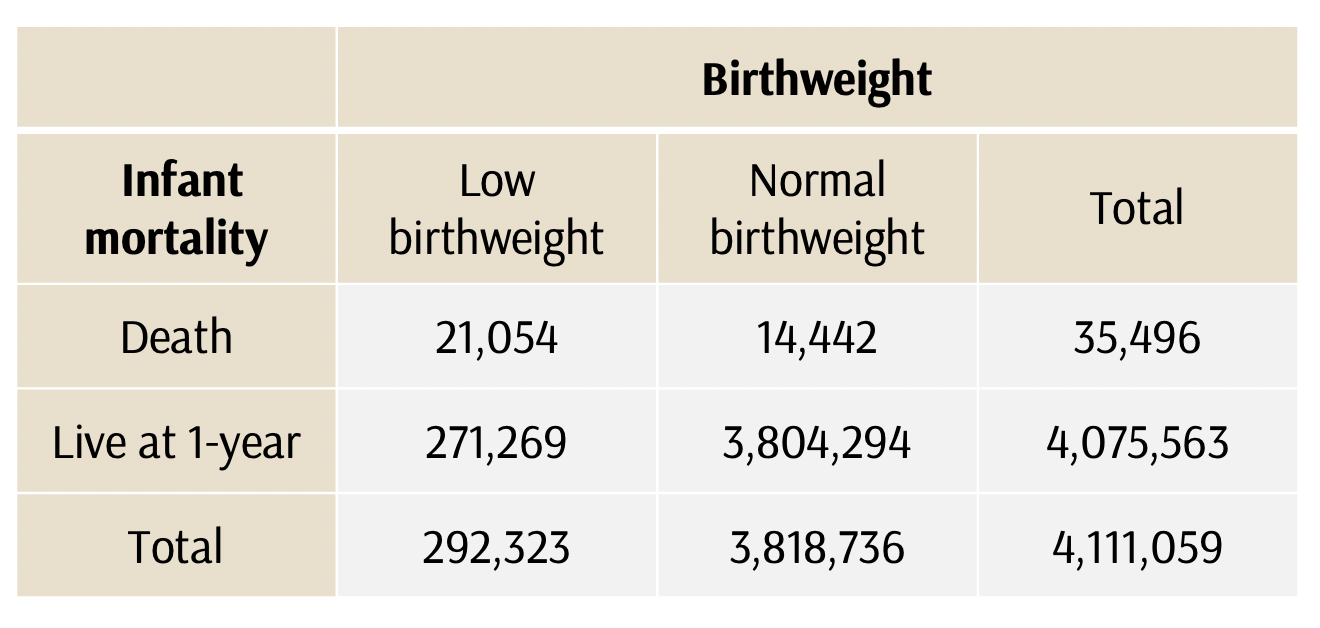
What is the conditional probability of an infant death, given that the child has a normal birth weight?
If A = death in first year; B=normal birth weight infant
P(A|B)
= 14,442 / (14,442+ 3,804,294)
= 3.8 deaths per 1,000 births
Conditional probability, A|B vs B|A
Or, if we wanted to use the conditional probability equation
P(A|B) = P(A and B)/P(B)
P(A and B) = 14,442
P(B)= 3,818,736
P(A|B) = 14,442/3,818,736 = 0.0038
* A= death in first year; B=normal birth weight infant
Conditional probability, A|B vs B|A
On the other hand, the conditional probability of P(B|A) is the probability that an infant had normal birth weight, given that the infant died within 1 year from birth
*B=normal birth weight infant; A = death in first year
Conditional probability, A|B vs B|A
Probability of A|B is 3.8 deaths per 1,000 births
Solve P(B|A) – the probability that an infant had normal birthweight, given that the infant died within 1 year from birth
P(B|A)
= 14,442 / (14,442+ 21,054)
= 0.41
4.1 normal birthweights of 1,000 baby deaths within 1 year from birth
*B=normal birth weight infant; A = death in first year
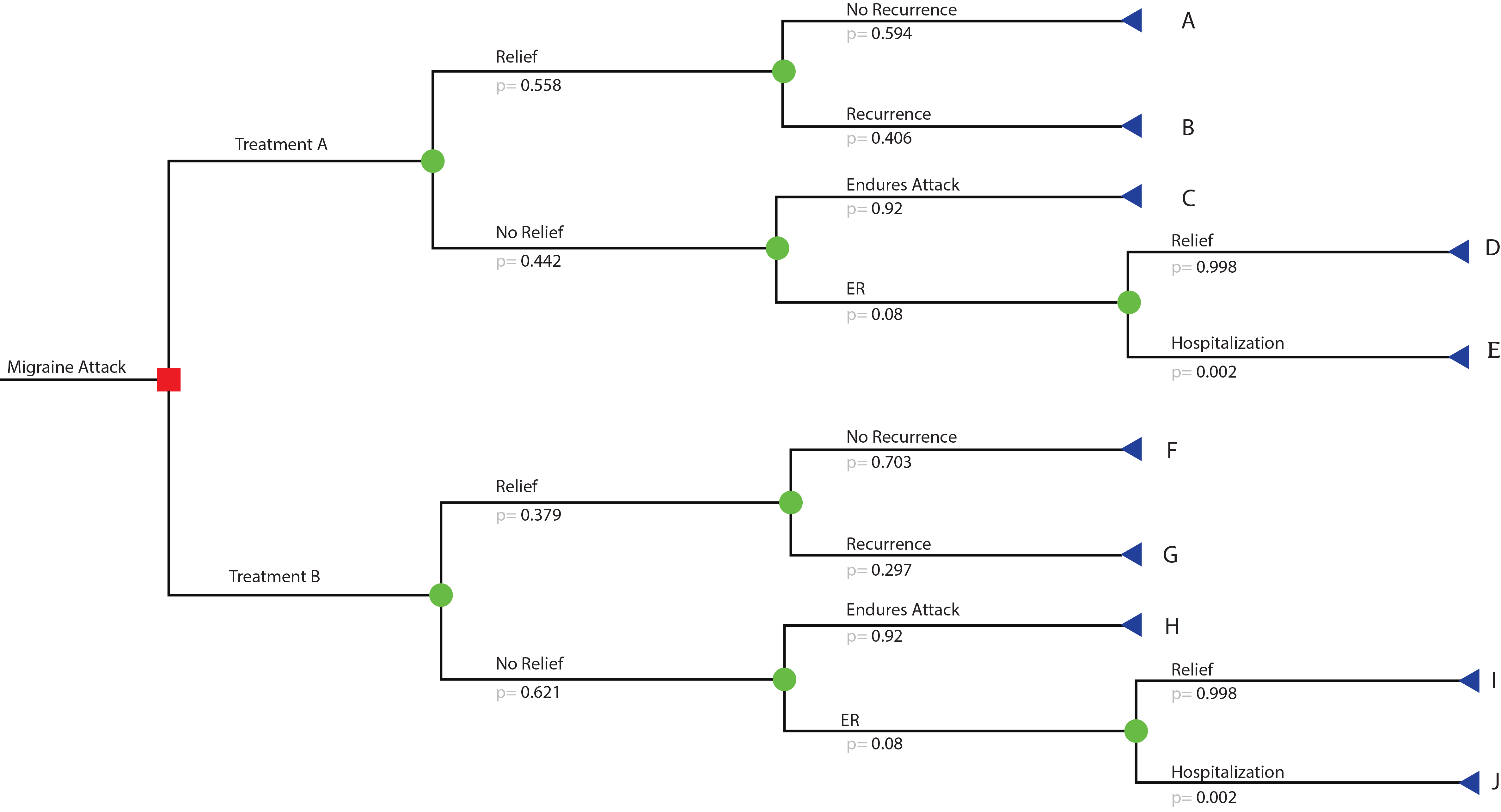
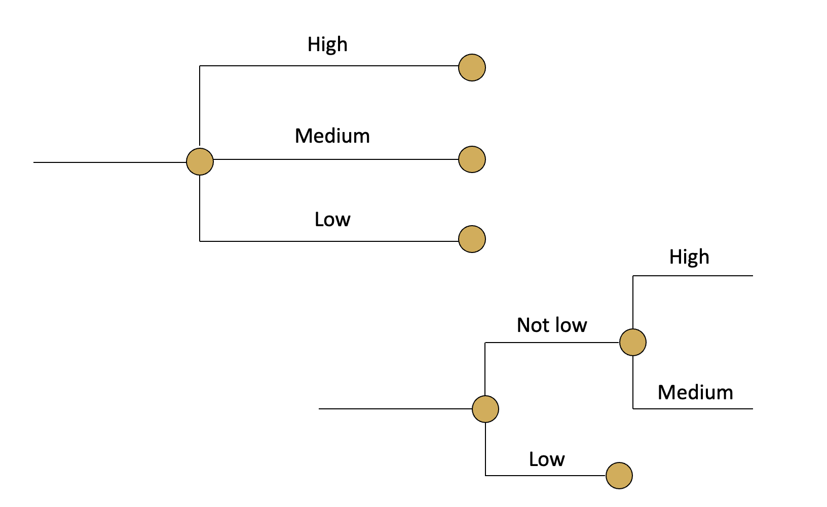
Some Do’s & “Dont’s”
- Two branches versus three
There is nothing inherently wrong with having three (or more) branches, as long as events are mutually exclusive and probabilities sum to 1.
However, additional branches increase model complexity & can complicate sensitivity analyses without necessarily adding insight.
Preview of what’s to come
More complex trees!