Probability review
Rates & Probabilities
Learning Objectives and Outline
00
Learning Objectives
Differentiate between rates and probabilities conceptually
Interpret rates and probabilities in applied examples
Identify and correctly interpret rates and probabilities in the literature
Outline
01
02
Rates review
03
Rates versus probabilities
04
Summary
05
Identifying rates and probabilities in the literature
06
Translating between rates and probabilities
Probability Review
01
Probability
Probability is the likelihood that an event occurs within a specified time period.
Out of everyone we followed for this period, what fraction experienced the event?
Probability can be reported in different ways
Proportion / percentage: 0.40 or 40%
Frequency: 40 per 100 (or 4 per 1,000)
Odds: P/(1-P) (ranges from 0 to \infty)
Epidemiologic terminology: - Cumulative incidence (risk): the probability of experiencing the event by time t - Examples: “1-year risk,” “5-year cumulative incidence”
Rates
02
Rates involve person-time
Incidence (hazard) rate: number of events per unit of person-time
Rates describe how fast events occur
Rates can range from 0 to \infinity
What is the difference between a rate and a probability?
Rates vs. probabilities
03
Rates vs. probabilities
Probability (risk): chance an individual experiences an event by a specified time
Rate: speed at which events occur per unit of person-time
Key distinction: rates use person-time in the denominator; probabilities do not
- **Probabilities collapse into a time window (10% by year 1; 30% by 3 years; it’s cumulative);
- **Rates have time in the denominator
Rate (incidence rate)
Probability (risk)
Example: same study, probability vs. rate
Study: 100 people followed for up to 4 years; 40 deaths.
Probability (risk) over 4 years: 40/100 = 0.40 ;
Interpretation: 40% died within 4 years.
Rate (if all 100 followed for 4 years): Total person-time = 100 \times 4 = 400 person-years; 40/400 = 0.10 deaths per person-year
Interpretation: 0.10 deaths occur for every 1 person-year of follow-up; or around 1 death per 10 person-years of follow-up across the study population
Timing & censoring
- Rates change when follow-up time differs, even if the number of events is the same
- Censoring or dropout reduces person-time and can increase the estimated rate
Example: events happen early vs. late
Study: 100 people, planned follow-up = 4 years
Case: 40 deaths occur in Year 1
- Person-time = (40 \times 1) + (60 \times 4) = 280 person-years
- Rate: 40/280 = 0.143 deaths per person-year
- Probability (risk): 40/100 = 0.40
When time-at-risk is not reported1
- When individual follow-up time is unavailable, events are often assumed to be evenly distributed
- This approximates equal person-time for everyone
- If events occurred earlier, the true rate would be higher (and vice versa)
Summary: Rates vs. Probabilities
04
Summary: Rates vs. Probabilities
- Probability
- Answers: What proportion of people experience the event by time X?
- Rate
- Answers: How fast do events occur, per unit of time at risk?
Summary: Rates vs. Probabilities
| Measure | Formula | Range | Used in |
|---|---|---|---|
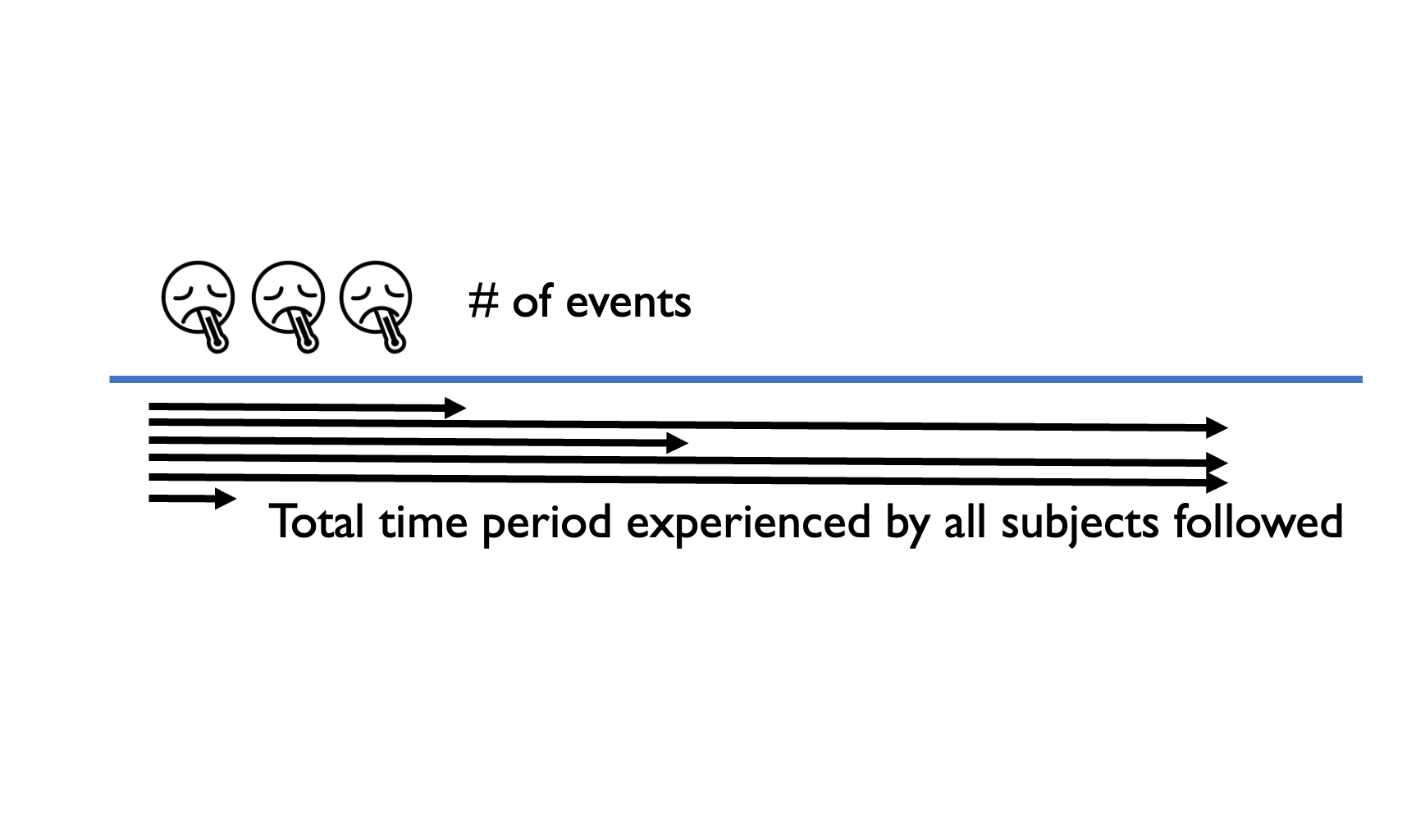
| Rate | \dfrac{\# \text{events}}{\text{total person-time}} | 0–\infty | Rate matrices |
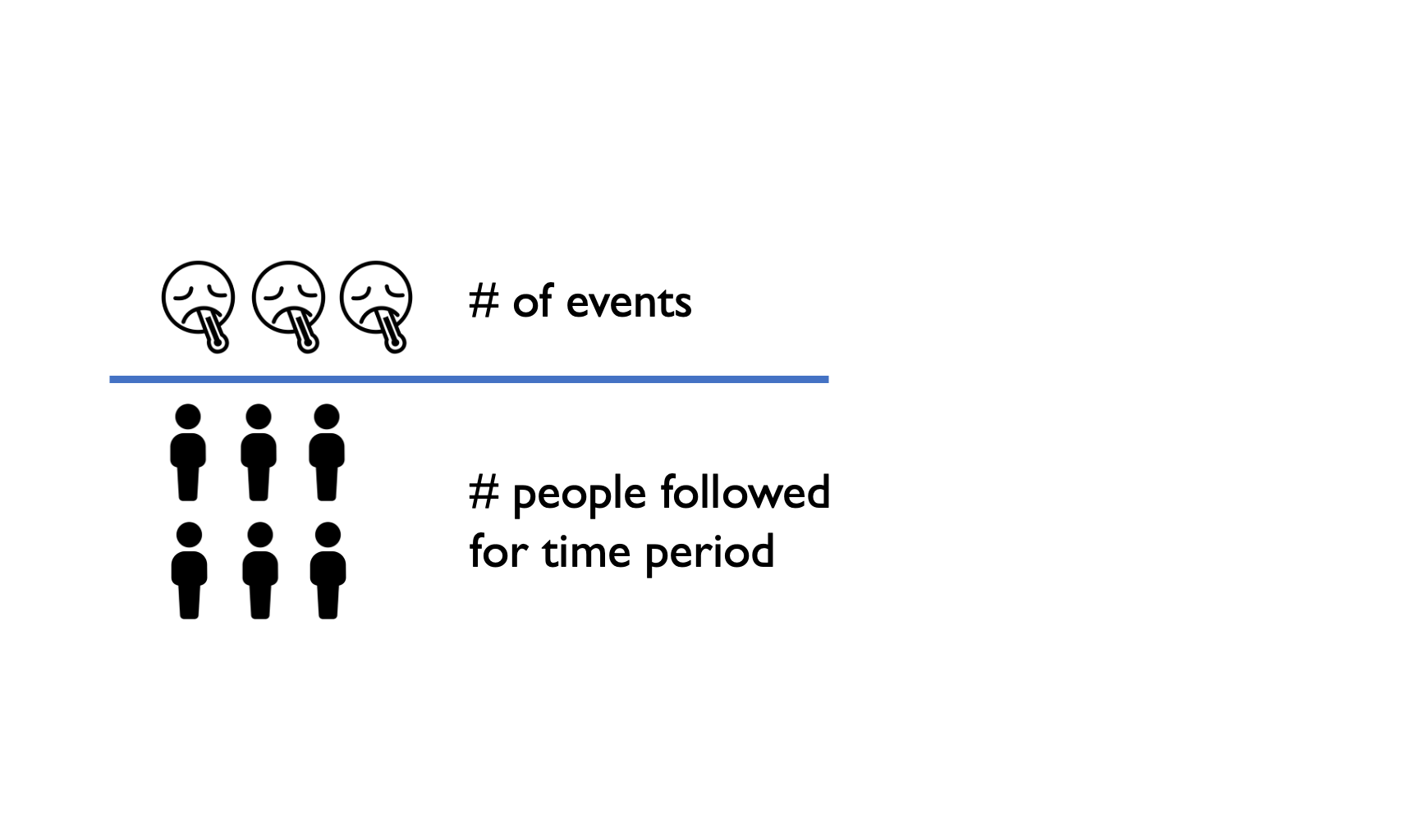
| Probability / risk | \dfrac{\# \text{events}}{\# \text{people followed}} | 0–1 | Probability matrices |
Identifying rates/probabilities through the literature
05
Identifying rates/probabilities through the literature
Identifying rates/probabilities through the literature
Translating between rates and probabilities
06
Converting rates/probabilities
- Rates are instantaneous; they represent the speed of an event happening & because speed scales linearly with time, you can multiply or divide rates when the time period changes.
- Probabilities are accumulated outcomes (they are cumulative & bounded between 0-1); they do not scale linearly with time. You can’t have more than 100% risk; so dividing/multiplying them does not preserve the correct relationship over time.
Another way of saying the same thing:
- A rate tells us how fast an event occurs; it scales with time.
- A probability tells us whether an event occurs within time “t”; it is cumulative & bounded. The relationship with time is non-linear because the chance of an event slows as fewer people remain at risk (i.e., why we say it’s “cumulative”)
Conversions
- A standard Markov model assumes an exponential (constant-hazard) process.
- This allows conversion between rates (instantaneous) and probabilities (over time).
- If the hazard changes over time, simple conversions no longer apply.
Rate to Probability p = 1 - e^{-rt}
Conversions
Probability to Rate
r = \frac{-ln(1-p)} {t}
Conversions
- exp(x): Applies continuous time accumulation (when converting rates to probabilities; the exponential ensures probabilities stay between 0 & 1 and that the timing of events is modeled correctly)
- ln(x): Removes it (when converting probability to rate)
Conversions
Example: Consider we have a 12-month probability of 10.8% that a child under age 6 is newly diagnosed with elevated blood lead levels. If your Markov model has a 3-month cycle length, a 3-month probability is needed.
Conversions
STEP 1 Convert the 12-month probability to a 12-month rate (or 12-month probability to a 3-month rate)
Note
Cannot divide/multiply probabilities
r = \frac{-ln(1-p)} {t}
r = \frac{-ln(1-.108)} {1} = 0.1142891
Note
Since the time period doesn’t change, the denominator is 1
Conversions
STEP 2 Convert the 12-month rate to a 3-month rate
\frac{0.1142891}{4} = 0.02857228
Conversions
STEP 2 Convert 3-month rate to 3-month probability
p = 1 - e^{-r\Delta t}
p = 1 - e^{−0.02857228∗1} = 0.028168
Conversions
OR, Step 1 Convert the 12-month probability to a 3-month rate
r = \frac{-ln(1-p)} {t}
r = \frac{-ln(1-.108)} {4} = 0.02857229
Conversions
STEP 2 Convert 3-month rate to a 3-month probability
p = 1 - e^{-r\Delta t}
p = 1 - e^{−0.02857229∗1} = 0.028168
Conversions
Note
***IF we took the probability of .108 / 4 to get the 3M probability, we would get 0.027. This is CLOSE but it could make a huge difference when modeling hundredths of thousands of individuals, for example
Alternative Rate-to-Probability Conversions
- Long cycles can include multiple transitions (healthy → sick → dead).
- Standard rate–probability conversion
p_{HS}= 1 - e^{-r_{HS}\Delta t}
treats transitions independently, ignoring competing risks. - This hides within-cycle events.
- Can underestimate deaths with long cycles.
- Fix: shorter cycles or competing-risk conversions.
Alternative Rate-to-Probability Conversions
A set of formulas often used to account for competing risks are as follows:
p_{HS}= \frac{r_{HS}}{r_{HS}+r_{HD}}\big ( 1 - e^{-(r_{HS}+r_{HD})\Delta t}\big )
p_{HD}= \frac{r_{HD}}{r_{HS}+r_{HD}}\big ( 1 - e^{-(r_{HS}+r_{HD})\Delta t}\big )
p_{HH} = e^{-(r_{HS}+r_{HD})\Delta t}
What to use
| Equation | Use case | Advantage |
|---|---|---|
| p = 1 - e^{-rt} | When you know a rate but need a probability for a fixed cycle length | Simple closed-form conversion under a constant (exponential) hazard |
| r = -\ln(1-p)/t | When you have a probability but need a rate to rescale across time intervals | Preserves the correct exponential relationship when changing cycle length |
| Competing-risk formulas p_{HS}, p_{HD} | When more than one event can occur from the same state (e.g., Healthy → Sick and Healthy → Dead) | Properly accounts for competing hazards and prevents hidden within-cycle events |
Alternative Rate-to-Probability Conversions
There’s an even more accurate way to correct for “competing risks” & while it’s beyond the scope of this introductory workshop, we will briefly review how to do this within the Markov lecture.
Key Takeaways
Rates & Probabilities
- Probabilities are cumulative and bounded (0-1)
- Rates are instantaneous and scale with time
- Conversions require a constant hazard assumption (hazard is flat within a time interval)